(Please note that the above page is best viewed on a pc, or device with a larger screen, not mobile. If you don’t see the date picker, zoom out until you do.)
As of writing (end July 2022), the test rig uses an uninsulated tank (an IBC) with 1m3 of water and two collectors with a total aperture area of 3.7m2. The tank is located outside so heat is lost overnight; therefore we can start again each day. The panels are pitched for collection in the winter, so the output reflects that.
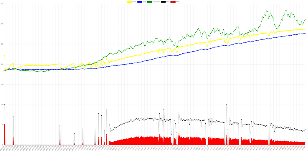
Explanation of graphs
Typically you can see a pattern of initial ‘teeth’ in yellow as the panel catches some morning sunlight and the starting temperature delta is exceeded. At this point, the panels are filled, but their temperature drops below the delta as that heat is removed and the sunlight is not enough to sustain it; the pump can’t run slowly enough to sustain flow without drain-back occurring. This process repeats until it is possible to maintain constant operation. Thereafter you can see that the panel temperature is clamped to within a few degrees of the tank output. You can see the pump speed modulating to achieve this, and the kW output changing constantly. We can thereby try to avoid start/stop cycling (‘short cycling’) which a constant speed drain-back system can suffer from when operating in marginal conditions.
Filling of the panels and pipework is determined by an optical sensor mounted in an inverse trap at the return point to the tank; modulation is allowed only when the panel and pipework are full. Occasionally, when flow rate is low, an unwanted drain-back event may start as air bubbles accumulate from the tank return. Typically this is detected and the bubbles purged – you might see this on the graph with a temporary increase in flow. Doing this has a danger of inducing hysteresis if the purge cycle runs for too long, but not doing so guarantees it!
Because the system can run in near syphon mode, pump power is reduced, and slower flow rates are possible. It’s this that allows operation in more marginal conditions than other drain-back systems. (Because we expect to run in this mode, we can use smaller diameter pipework that is more appropriate to household installation – typically 22mm diameter.)
Location
There are large trees to the immediate east of the test rig; morning sunlight is restricted. Prague sees an average of 1670 hours of sunlight per annum. Summer temperatures can be high (sometimes approaching 40c) and winter cold (sometimes -20c).
Graphs
The graphs you see are created as follows: Sensor data from remote modules is requested via RS485, using our own lightweight protocol, from the master module. Optimal pump speed is calculated by the master module and transmitted back to the pump module in the same manner. Feedback from the pump is again collected by the master. Every 20 seconds or so logging data is transmitted by the master to a pc where our logging daemon runs. Three samples are collected, and their middle values are written to a csv log about every minute. That log is then uploaded to our server & the process repeats.
When you view the log page, you run a script that downloads the csv file and plots it in your browser. Only ‘Bank 0’ is operational at the moment. If you have checked ‘Auto refresh’, the graph will update throughout the day. Metrics are shown at the bottom of the page: you can enter the price per kWh that you expect to pay for water heating..
E. & O. E.